This tutorial covers advanced features of Covasim, including custom population options and changing the internal computational methods.
Click here to open an interactive version of this notebook.
Defining populations with SynthPops
For complex populations, we suggest using SynthPops, a Python library designed specifically for this purpose. In contrast the population methods built-in to Covasim, SynthPops uses data to produce synthetic populations that are statistically indistinguishable from real ones. For a relatively complex example of how SynthPops was used to create a complex school network for the Seattle region, see here.
Defining contact layers
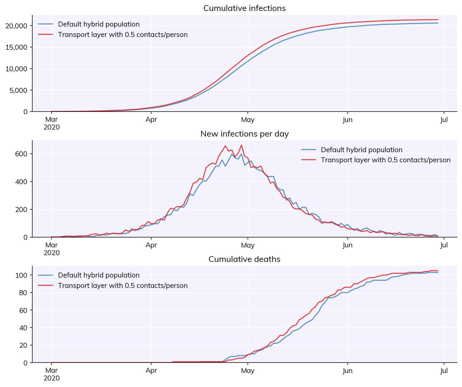
As mentioned in Tutorial 4, contact layers are the graph connecting the people in the simulation. Each person is a node, and each contact is an edge. While enormous complexity can be used to define realistic contact networks, a reasonable approximation in many cases is random connectivity, often with some age assortativity. Here is an example for generating a new contact layer, nominally representing public transportation, and adding it to a simulation:
import numpy as npimport covasim as cvcv.options(jupyter=True, verbose=0)# Create the first simorig_sim = cv.Sim(pop_type='hybrid', n_days=120, label='Default hybrid population')orig_sim.initialize() # Initialize the population# Create the second simsim = orig_sim.copy()# Define the new layer, 'transport'n_people =len(sim.people)n_contacts_per_person =0.5n_contacts =int(n_contacts_per_person*n_people)contacts_p1 = cv.choose(max_n=n_people, n=n_contacts)contacts_p2 = cv.choose(max_n=n_people, n=n_contacts)beta = np.ones(n_contacts)layer = cv.Layer(p1=contacts_p1, p2=contacts_p2, beta=beta) # Create the new layer# Add this layer in and re-initialize the simsim.people.contacts.add_layer(transport=layer)sim.reset_layer_pars() # Automatically add layer 'transport' to the parameters using default valuessim.initialize() # Reinitializesim.label =f'Transport layer with {n_contacts_per_person} contacts/person'# Run and comparemsim = cv.parallel(orig_sim, sim)msim.plot()
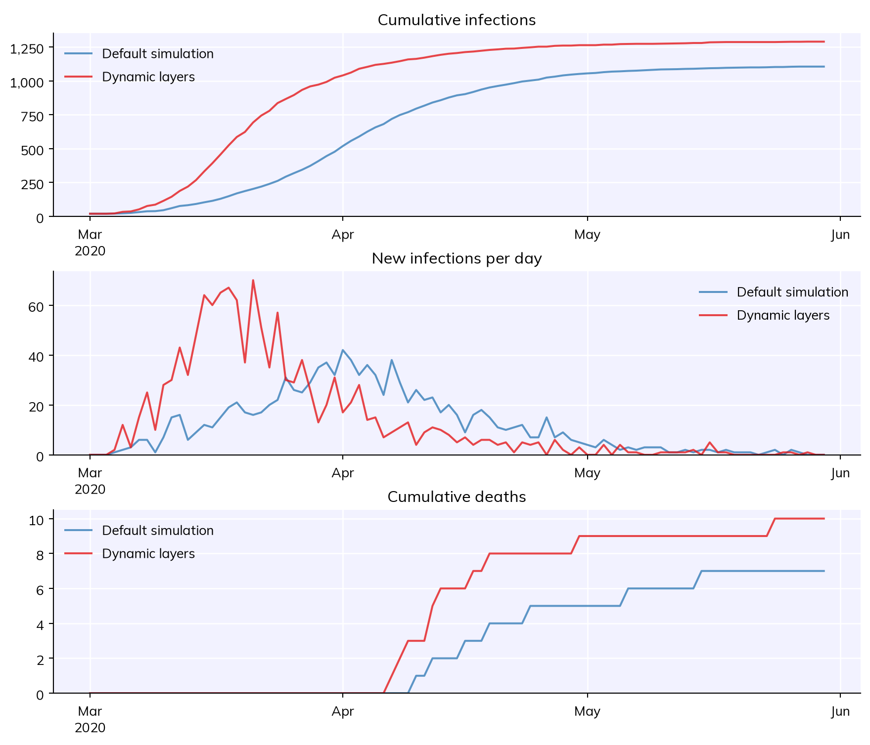
You can also define custom layers that update dynamically, e.g. based on a supplied number of contacts per day. To do this, create a new Layer class and define the step() method, which is called on each timestep; the contacts are stored in self.edges. For example:
import covasim as cvimport numpy as npimport sciris as scclass CustomLayer(cv.Layer):''' Create a custom layer that updates daily based on supplied contacts '''def__init__(self, contact_data, **kwargs):''' Store the contact data '''super().__init__(**kwargs)self.contact_data = contact_datareturndef step(self):''' Update the contacts ''' uids =self.sim.people.indices() # The people who are alive n_new =self.contact_data[self.ti] # Pull out today's contactsself.edges.p1 = uids[cv.choose_r(max_n=len(uids), n=n_new)] # Choose with replacementself.edges.p2 = uids[cv.choose_r(max_n=len(uids), n=n_new)] # Paired contactself.edges.beta = np.ones(n_new, dtype=cv.default_float) # Per-contact transmission (just 1.0)return# Define some simple parameterspars = sc.objdict( pop_size =1000, n_days =90,)# Create the custom layer, to use instead of the default one ('a')contact_data = np.random.randint(pars.pop_size*10, pars.pop_size*20, size=pars.n_days+1) # Generate a number of contacts for each daylayer = CustomLayer(contact_data, name='a')# Set up and run the simulationbase_sim = cv.Sim(pars, label='Default simulation')sim = cv.Sim(pars, networks=layer, label='Dynamic layers')# Run and plotmsim = cv.parallel(base_sim, sim)msim.plot()
Exception ignored while finalizing file <_io.BytesIO object at 0x7f797850bec0>:
Traceback (most recent call last):
  File "/opt/hostedtoolcache/Python/3.14.8/x64/lib/python3.14/site-packages/starsim/utils.py", line 667, in __getattr__
    def __getattr__(self, attr):
BufferError: Existing exports of data: object cannot be re-sized
Defining custom population properties
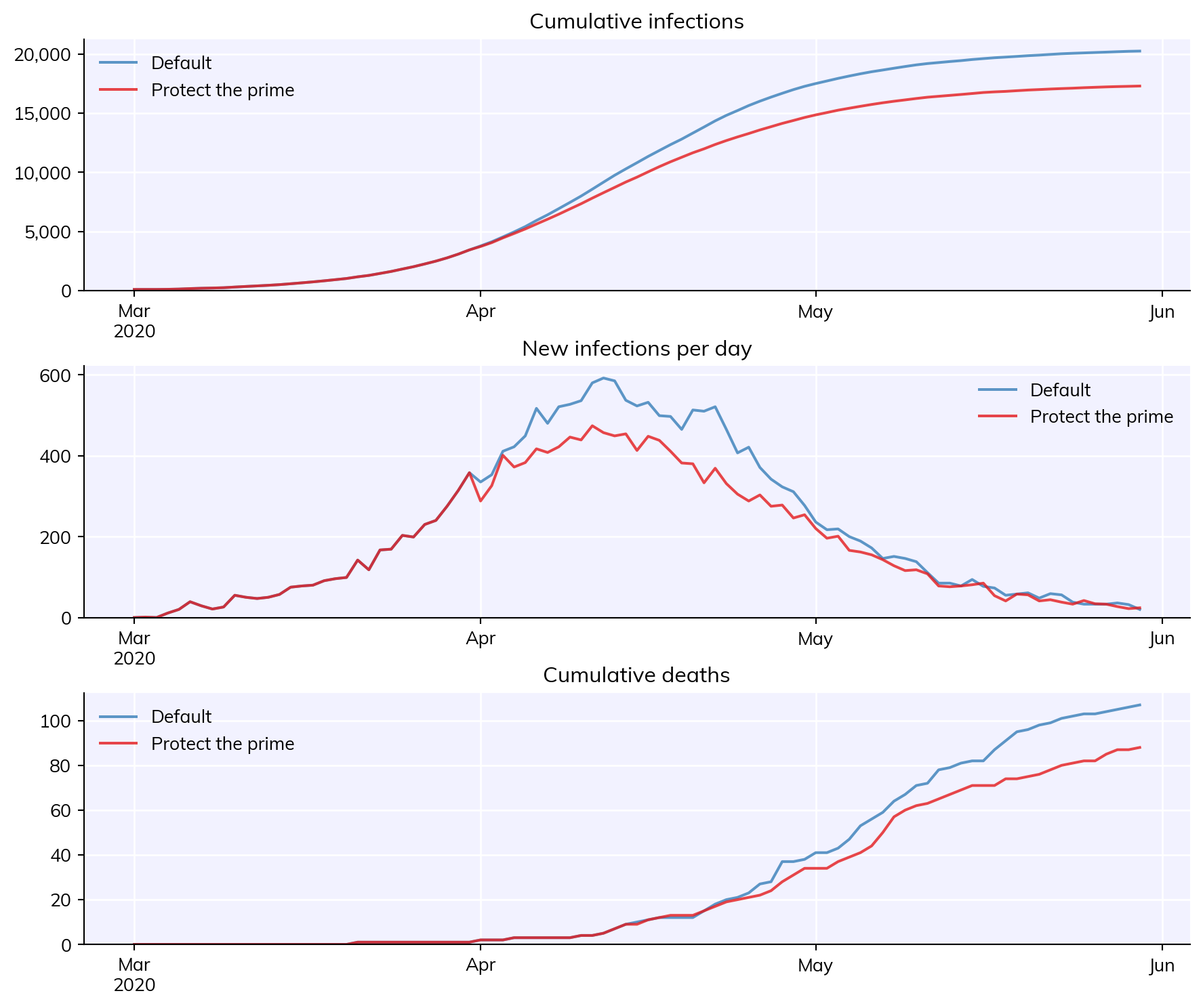
Another useful feature is adding additional features to people, for use in subtargeting. For example, this example shows how to define a subpopulation with higher baseline mortality rates. This is a simple example illustrating how you would identify and target people based on whether or not the have a prime-number index, based on the protecting the elderly example from Tutorial 1.
import numpy as npimport sciris as scimport covasim as cvdef protect_the_prime(sim):if sim.ti == sim.day('2020-04-01'): are_prime = sim.people.prime sim.people.rel_sus[are_prime] =0.0pars =dict( pop_type ='hybrid', pop_infected =100, n_days =90, verbose =0,)# Default simulationorig_sim = cv.Sim(pars, label='Default')# Create the simulationsim = cv.Sim(pars, label='Protect the prime', interventions=protect_the_prime)sim.initialize() # Initialize to create the people arraysim.people.prime = np.array([i for i inrange(len(sim.people)) if sc.isprime(i)]) # Define whom to target, by their index# Run and plotmsim = cv.parallel(orig_sim, sim)msim.plot()
Changing Numba options
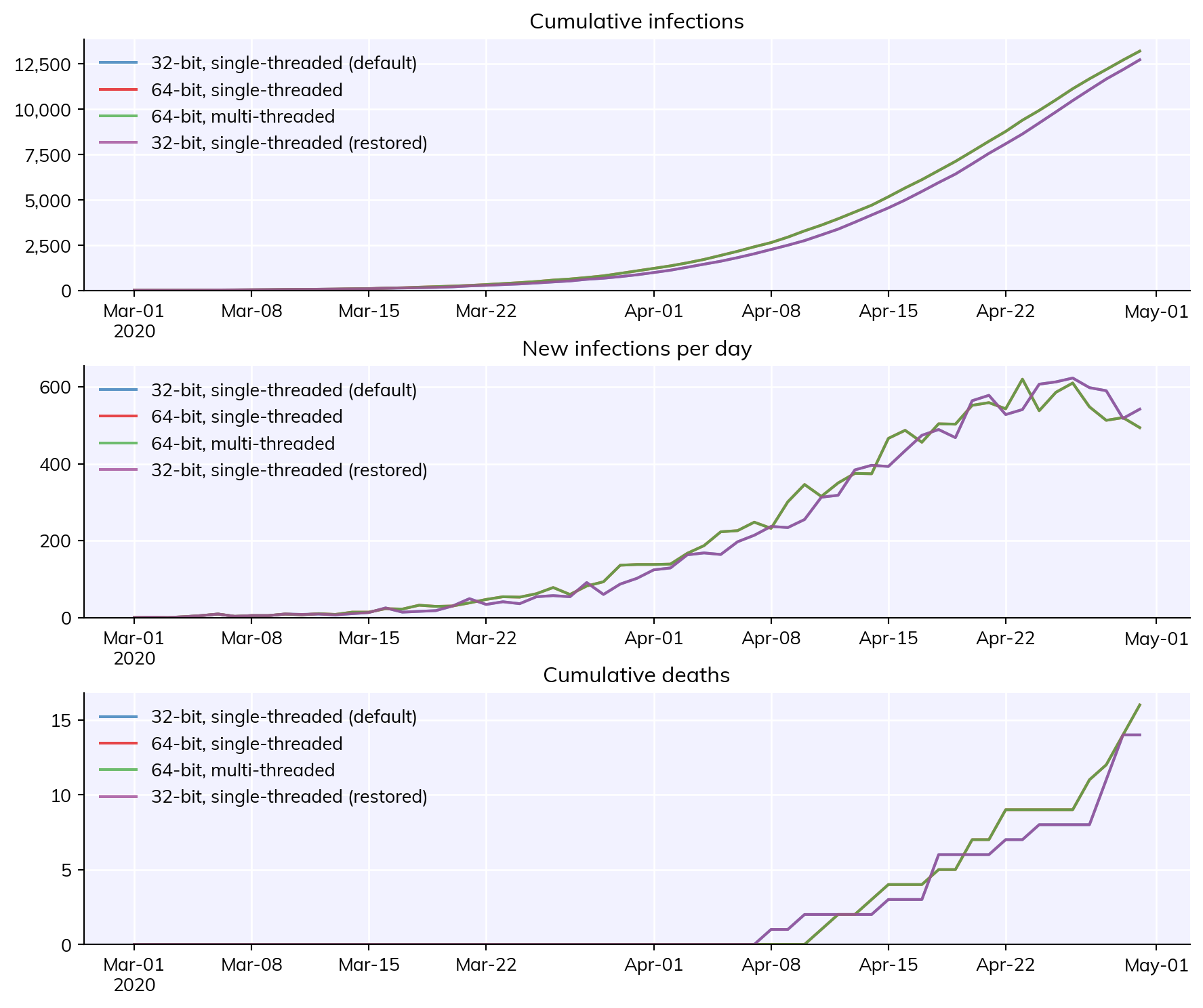
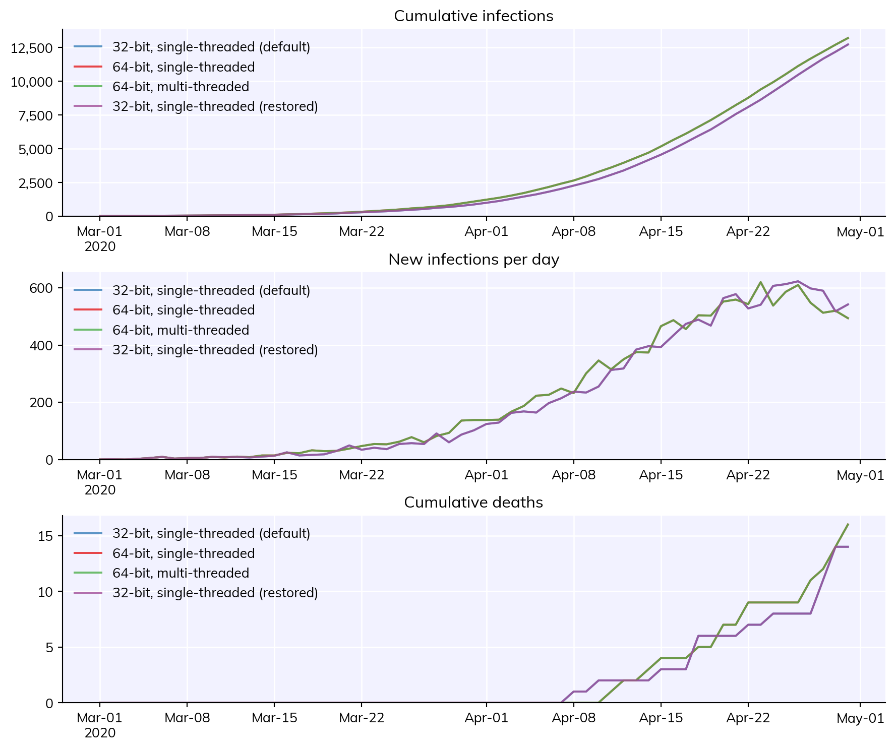
Finally, this example shows how you can change the default Numba calculation options. It’s not recommended, but it’s there if you want it.
import covasim as cv# Create a standard 32-bit simulationsim32 = cv.Sim(label='32-bit, single-threaded (default)', verbose='brief')sim32.run()# Use 64-bit instead of 32cv.options.set(precision=64)sim64 = cv.Sim(label='64-bit, single-threaded', verbose='brief')sim64.run()# Reset to defaultscv.options.set('defaults')sim32b = cv.Sim(label='32-bit, single-threaded (restored)', verbose='brief')sim32b.run()# Plotmsim = cv.MultiSim([sim32, sim64, sim32b])msim.plot()